upTimer 3.0

I think it was in 2005. I was looking around for some sort of hardware component Timer to track Podcast recording session elapsed time. I came across an Ad in Radio Magazine sponsored by ESE. They specialize in manufacturing different types of clocks, timers, and timecode utilities intended for broadcast environments. It was their Up Timer (designed to track live programs and air time) that sparked my interest.

The device originally retailed for (I think?) $300. Functionality is straightforward: LED display – Start, Stop. Reset buttons, and a DB9 interface for remote control operation. Interestingly – it is limited to a 60 min. ceiling. Actually, it’s range was/is 00:00 – 59:59.

Below is a snapshot of the current (desktop) model. It retails for less than $200.

Anyway, shortly after my initial discovery of the device, I decided to build a software version for the Mac. Version 2 was released in 2011. Seven years later I am releasing Version 3.

Besides the noticeable UI redesign, the application is now 64bit.

* The ceiling is somewhat flexible, thus allowing the user to select either a 60 or 90 min. ceiling.

* The upTimer font color can be set to blue or yellow. The font color shifts to red when the elapsed time reaches the 2 min. mark relative to the defined ceiling.

* The operation keys (Reset, Stop, Start) are mapped to ←, ↓, → keyboard keys respectively.

* The application window checks in at approx. 735 x 340 pixels. I plan to add scalability to the UI sometime in the future.

Note in this version I decided to include and display a running long form Date and Time string above the upTimer. The user can hide it’s visibility, along with the linked ceiling setting indicator.

Update: Version 3.5 includes a new UI size display preference. The Large option resizes the application window by approx. 40%.

Update: Version 3.5.1 includes Application Menu actions with mapped keyboard shortcuts to toggle the display size of the UI.

Update: Version 3.5.2 mainly includes UI tweaks.

Download upTimer 3.5.2
(OSX 10.10.5 or later)

Fee? None. My only request is to please keep me in mind for expert Podcast Audio Post, audio processing, and consulting. I’ve been in the space since 2004.

-paul.

Mic Preamp Level and Gain Staging

When configuring voice processors such as the dbx 286A/s (or any other device with a similar configuration) – there is always an optimal preamp level setting or sweet spot for the connected microphone. Basically – your mic needs to be properly driven at the preamp stage in order to pass sufficient gain with low inherent noise and ample headroom throughout the device and thru it’s downstream processing modules.

In general, intra-device Drive based Compressors are designed to elevate the module input gain as the setting is increased. In doing so the dynamic range of the passing signal will be decreased. This often results in an elevation of the noise floor that was nonexistent prior to the compression stage.

Please note: After initial preamp optimization, this setting should remain static. The preamp level control should NOT be used for gain staging or compression noise floor compensation! In essence improper preamp gain will hinder the effectiveness of downstream intra-device processing.

My recommendation for optimal signal to noise: set the preamp gain accordingly. Apply intra-device processing. Lastly, use the OUTPUT gain for any necessary gain staging or compensation. This will have no effect on the initial (and hopefully optimized) mic input setting as well as the subsequent processed signal passing through the device.

-paul.

Aphex 320D Compellor

What is a Compellor? In short it is a Compressor-Leveler-Limiter. The device is specifically designed for the transparent control of audio levels.

It operates as a stereo processor or as a two-channel (mono) processor supporting independent channel control.

The device includes 3 interactive gain controllers:

– Frequency Discriminate Leveler
– Compressor
– Limiter

Additional features include a Dynamic Release Computer (DRC), Dynamic Verification Gate (DVG), and a Silence Gate.

The original device (model 300 Stereo Compellor) was released in 1984. The product line evolved and culminated in 2003 with the release of the 320D. Through the years the Compellor has been widely used in professional broadcast, post houses, recording studios, and live venues.

In 2004 I purchased a used model 320A from a radio station. The “A” reference indicates it’s analog circuitry. I’ve used the 320A for countless audio file and tape transfers, post production processing, Telephone/Skype recording sessions, and monitoring. The device provides three selectable Operating Levels … +8dBu, +4dBu, and -10dBV.

Recently the complex level and gain reduction metering for the right channel failed. I replaced the faulty 320A with a 320D. This version features digital and analog I/O with common selectable (analog) Operating Levels (+4dBu, and -10dBV).

At some point my faulty 320A will be shipped out to Burbank California for authorized service.

320D – Automatic Processing and Detection

As noted Aphex classifies the Compellor as a Frequency Discriminant Leveler. It responds slower and less aggressively to low frequencies. In essence low frequency energy will not initiate gain reduction.

A Dynamic Release Computer (DRC) instantiates program dependent compression release times.

The Dynamic Verification Gate (DVG) computes the historical average of peak values and verifies whether measured values exceed or are equal to the historical value. When the signal level is below the average, leveling and compression gain reduction is frozen.

Controls

The device Drive control sets the preprocessed VCA gain. Higher settings yield a higher level of gain reduction (VCA refers to Voltage Controlled Amplifier).

The Process Balance control allows the operator to fine tune the Leveling and/or Compression balance and weighting. Leveling is a slow method of gain reduction. It maintains transient retention and wider dynamics. The Compression stage works faster and acts more aggressively on inherent dynamics. The key is by combining both modes, the processed output will be very consistent

A Rate (speed) toggle option is provided: Fast, suitable for speech/voice, or Slow, suitable for program material such as produced TV and/or Radio programs.

The device Output control normalizes the processed audio to 0VU.

Silence Gate: Aphex stresses – this is not an audio gate! It is a user defined threshold parameter. When the signal drops below the threshold for 1 sec. or longer, the Silence Gate freezes the VCA gain. This prevents the buildup of noise during pauses and/or extended passages of silence.

The device Limiter features a very fast attack and high threshold. It is designed to prevent occasional high transient activity and overshoots.

A Stereo Enhance mode is available on the 320A and 320D models. When activated it widens the stereo image. It’s effect is dependent upon the amount of applied compression.

Metering

The 320D Compellor features three, bi-color (red, green) LED metering modes: Input, Output, and Gain Reduction. For Input/Output metering – the red LED’s indicate VU/average. Green LED’s indicate peak level.

When the meter is set to display gain reduction (“GR”), the green LED’s indicate total gain reduction. Depending on the Process Balance control weighting – a floating red LED may appear within green LED instances. The floating red LED indicates Leveling gain reduction. If Leveling gain reduction is in fact occurring, the total gain reduction will be indicated by the subsequent green LED(s).

Below are 4 examples:

Example 1 displays Input or Output metering with an average (red) level of 0VU and a peak (green) level of +6dB. This translates to a +4dBu average level and a +10dB peak level (analog OL set to +4dBu).

Example 2 displays 4dB of Leveling Gain Reduction and 8dB of Total Gain Reduction.

Example 3 displays 12dB of Leveling Gain Reduction.

Example 4 displays 10dB of Compression Gain Reduction.

**Notice the position of the Process Balance control for examples 2, 3, and 4.

320D I/O

The 320D is essentially an analog processor utilizing standard XLR I/O jacks. The device also includes AES/EBU XLR jacks along with an internal DAC for digital I/O. The Input mode and/or Sample Rate is user selectable.

When implementing digital I/O – the Incoming audio is converted to analog as it passes through the device. The audio is then converted back to digital and output accordingly.

The digital input is calibrated internally and matches -20dBFS to 0VU on the Compellor’s meter. The +4dBu/-10dBV Operating Level options only affect the analog I/O.

Notes:

The Aphex Compellor is a long standing, highly regarded, and ubiquitous audio processor. It has been an integral multipurpose tool for me for 12+ years. My newly purchased (used) 320D is in near mint condition. In fact it looks and feels as if it was hardly used by the previous owner.

My system includes additional Aphex audio processors (651 Compressor, 109 EQ, 622 Expander/Gate, and a 720 Dominator II Multiband Peak Limiter). As well, a Mackie Onyx 1220i Mixer, Motu I/O, dbx 160A Compressor, dbx 286A Mic Processor, Marantz CF Recorder, and a Telos One Digital Hybrid. All components, with the exception of the 286A – are interfaced through a balanced Patchbay.

A typical processing/monitoring chain will pass system audio through the Compellor, followed by the 720 Peak Limiter. The processed audio is ultimately routed to the system’s Main Output(s). This chain optimizes playback of poorly produced Podcasts, VO’s, live streams, or videos. The routing is implemented via Patchbay.

A typical audio processing chain will route Pro Tools audio out via hardware insert (or bus, alternative output, etc.) through the Compellor (or a more complex chain) and returned in Pro Tools. In this scenario I use a set of assignable interface line inputs/outputs. The routing is implemented via Patchbay. I document the setup and use of hardware inserts here.

-paul.

Recording Multiple Skype Clients On A Single Host System

**UPDATE 1: It appears current versions of Skype (e.g. ver.8.12.0.14) broke the capability to run multiple instances of Skype (via command line) on a Mac. I’m looking into a fix. You can use Source-Connect Now as a high quality Skype alternative. Two accounts will be necessary. Setup and Routing will be consistant with what is described in this documentation. Please contact me with questions …

**UPDATE 2: I solved the incompatability issue noted above by uninstalling Skype 8.xx for Mac and reverting back to Skype ver. 7.58 (501). Once again it is possible to run multiple instances of Skype (discrete accounts) on the host system by executing the terminal command noted in this documentation …

**UPDATE 3: It is now possible to run multiple instances of Skype 8.xx (discrete accounts) on the host system. I coded a Cocoa application capable of launching the discrete accounts. Contact me for details …

* * *

It is possible to record two (or more) independently connected Skype clients on discrete tracks on a single computer in RT. The workflow requires independent Mix-Minus feeds configured in a supported DAW such as Pro Tools or Logic Pro.

Plausible Session Senarios:

(Scenario A) Typical Podcast consisting of a Host + Skype Guest + Skype Guest. Dual Mix-Minus feeds are implemented in the Host’s DAW. All participants recorded on discrete tracks in RT utilizing two individual incoming Skype clients running simultaneously on the Host system.

(Scenario B) Engineer + Skype Session Participant + Skype Session Participant. Dual Mix Minus feeds are implemented in the Host’s DAW. Both participants recorded on discrete tracks utilizing two individual incoming Skype clients running simultaneously on the Host system.

Scenario B describes an engineering session providing support for independently located remote Skype participants who seek recording and post services. The workflow frees the participants from recording responsibilities and file management.

As noted both Scenarios require the use of two individual Skype clients running simultaneously on the Host/Engineer’s system. This concept is publicly documented using various methods.

What differentiates my workflow is the use of virtual routing within the Recording Session on a single machine. Dual Mix-Minus feeds are implemented in the Host’s DAW with zero dependency on hardware Aux Sends.

Loopback by Rogue Amoeba is used to create Virtual Devices and Pass-Thru’s. They will be encapsulated in an Aggregate Audio Device created in OSX. Additionally, my working Motu Audio Interface (8×8) will be added to the Aggregate Device for maximum flexibility.

Dual Mix-Minus

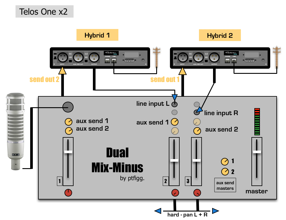
The intent of a single Mix-Minus feed is to send a Host’s audio back to a Session participant. This is commonly implemented on a hardware mixer or console using an Aux Send. It is nothing more than a discrete audio output with a level control.

When adding a second participant, the Host’s audio is routed to both participants using two Aux Sends (A), (B). The implemented Sends are also used to establish communication between the included participants.

For example:

Send (A) contains the Host + Participant 1 —-> signal is routed to Participant 2
Send (B) contains the Host + Participant 2 —-> signal is routed to Participant 1

Virtual Device Creation

The following I/O configuration is necessary for the described Host/Engineer + Skype 1 + Skype 2 scenario:

3 Mono Inputs: [Host] + [Skype Client 1] + [Skype Client 2]
2 Mono Outputs: [Host/Skype Client 1] + [Host/Skype Client 2]

Additional output routing will be necessary for monitoring and external recording. We will address this in a moment.

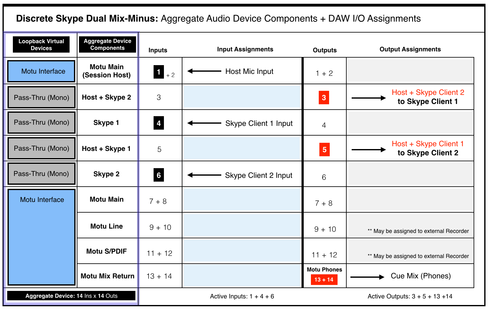
Please review the following I/O Matrix table:

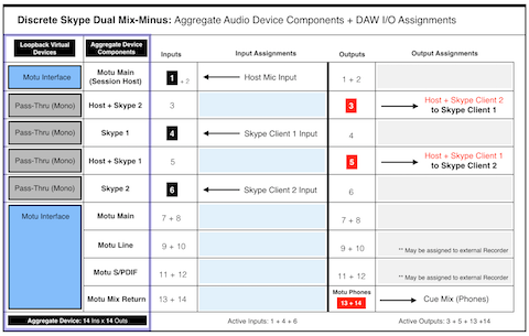
Column 1 lists six Virtual Devices created in Rogue Amoeba’s Loopback application. Column 2 lists their associated user defined names.

• An initial Motu Audio Interface instance is created with inputs/outputs 1+2 mapped for use. Input 1 will represent the Host Mic.

• Four individual (Mono) Pass-Thru Devices are created:

Input 4 will be mapped to Skype Client 1
Input 6 will be mapped to Skype Client 2

Output 3 will include [Host + Skype Client 2]
Output 5 will include [Host + Skype Client 1]

• A secondary Motu instance is created with all available inputs/outputs mapped for use (8×8 by default). This will supply additional routing flexibility for monitoring and external recording. In fact the I/O Matrix table displays the use of outputs 13+14 for the Cue Monitor Mix (Phones).

Note the Inputs and Outputs are purposely alternated to prevent direct patching and subsequent feedback.

These user defined Loopback Virtual Devices will appear in the Mac OSX Audio MIDI Setup utility. They can be used individually. They can also be combined, thus creating a cumulative (Aggregate) Audio Device. We will utilize both options (individual Virtual Devices for Skype Clients + cumulative Aggregate as the DAW’s default I/O).
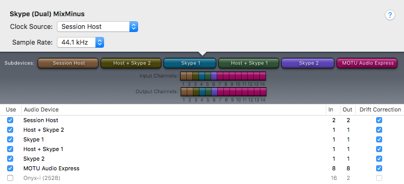
Aggregate Device

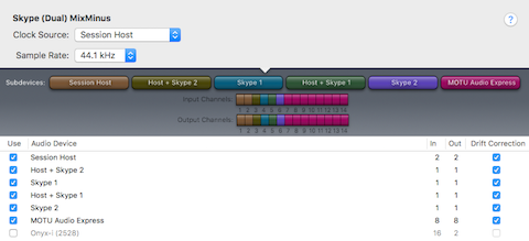
The image below displays a user defined Aggregate Audio Device created in OSX using the Audio MIDI Setup utility. It is named Skype (Dual) MixMinus. Notice how I’ve selected the Virtual Devices created in Loopback as Subdevices. Also notice how each Subdevice accurately displays input and output I/O mapping for a total of 14 inputs + 14 outputs. This matches the configuration displayed in the I/O Matrix table diagram above. The Aggregate Audio Device is now ready for DAW integration.

DAW Implementation

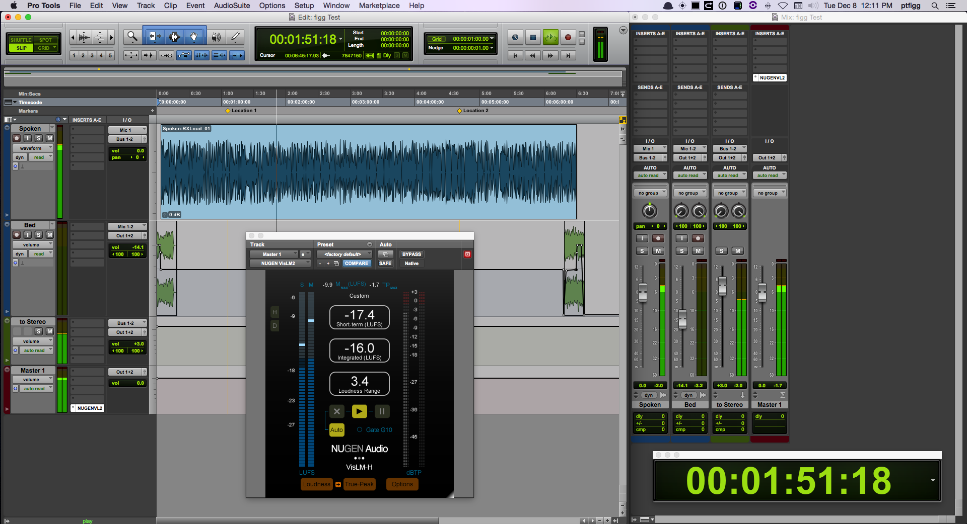
For this demonstration I will be using Pro Tools with the Skype (Dual) MixMinus Aggregate set as the Playback Engine (it’s default Session I/O). This configuration has also been successfully implemented in Logic Pro X. It has not been tested in Adobe Audition.

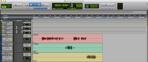
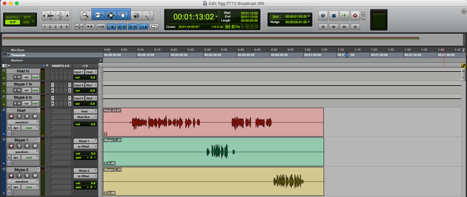
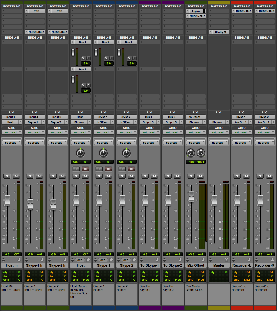
The Chanel Strip configuration will be described in sequential order. Please note the described Session configuration is more complex than what is required.

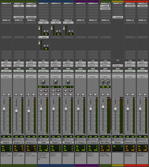
The first 3 Channel Strips (Green) are mono Auxiliary Inputs. Their assigned Inputs are the Host Mic, Skype Client 1, and Skype Client 2. Notice how the assigned inputs match the input configuration as displayed in the I/O Matrix table diagram (1 + 4 + 6).

The Faders on these Channel Strips function as input level controllers for each source input before the signals reach the pre-fader recording tracks.

Two audio plugins are inserted on each Skype Client input Channel Strip (Downward Expander and Limiter). The Expanders will transparently attenuate the inactive input. The Limiters will function as a safeguard thus preventing unexpected signal level overload. Plenty of headroom is maintained. In essence the Limiters will rarely engage.

Tracking Configuration

The outputs of the source input Channel Strips are routed (via virtual Buses) to the inputs of 3 standard mono Audio Channel Strips (Blue). When armed, they will record the source inputs discretely.

Sends

The Host Channel contains 2 active Sends passing audio to Bus 1 and Bus 2.
The Skype 1 Channel contains 1 active Send passing audio to Bus 2.
The Skype 2 Channel contains 1 active Send passing audio to Bus 1.

Returns

2 additional Auxiliary Input Channel Strips (Purple) receive signal from Send Buses 1 + 2.

Configuration as follows:

• The To Skype-1 input is set to Bus 1. This Bus includes the tapped Host audio and the tapped Skype 2 client audio. It’s output is set to Output 3.

• The To Skype-2 input is set to Bus 2. This Bus includes the tapped Host audio and the tapped Skype 1 client audio. It’s output is set to Output 5.

Notice how the assigned outputs (3 + 5) match the output configuration displayed in the I/O Matrix table diagram.

At this point we’ve created a dual Mix-Minus in the mixer…

* * *

Monitoring and Pan Offset

Pro Tools attenuates center-panned mono tracks according to a user defined Pan Depth setting. My setting is always -3 dB.

Here’s how I reconstitute the attenuation:

Notice the outputs of the Skype 1 and Skype 2 audio tracks are routed to a stereo Bus labeled to Offset. An Auxiliary Input Channel Strip (Green, labeled Mix Offset) receives the audio from the to Offset virtual Bus. I use the Channel Strip fader to add +3 dB of static gain to reconstitute the previously applied attenuation on the passing signal.

The Mix Offset Channel Strip’s output is set to Phones. This signal path represents the Interface Headphone outputs (13+14). They are referenced in the I/O Matrix table diagram.

The Master Fader’s (Yellow) output is also set to Phones. This configuration allows the engineer to monitor the Skype participants via headphones connected to the Motu Interface.

Notice the output for the Host Audio Track is set to Mute Bus. This is an unassigned virtual Bus. The Host Mic input is directly monitored (also via headphones) through the Motu Interface. Setting the Host channel output to the Session’s Phones output Bus will blend the hardware monitored mic signal with the slightly latent Session output. Using the unassigned Bus solves this. Of course in Post the hardware monitored signal will be absent. In this case the output must be reassigned to the Phones output Bus.

Skype

In preparation for recording, two independent instances of Skype (using unique accounts) must be launched on the Host System.

My Preferred method:

1) Launch Skype as normal and login to your primary account.

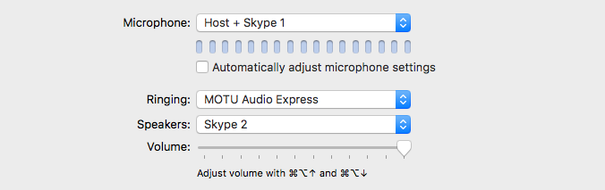
2) In the Skype Preferences/Audio/Video – define the Microphone (input) and Speakers (output) as displayed:

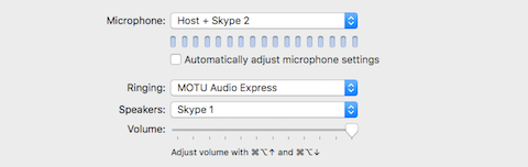
Notice we revert back to independent Virtual Devices created in Loopback for the configuration of this Skype instance. The Host + Skype 2 device is essentially output 3 in the configured DAW. It passes the Host + Skype Client 2 audio to this running instance of Skype.

[Speakers: Skype 1] is mapped to input 4, previously assigned in the DAW’s configured Session.

3) To launch the second instance of Skype – run the OSX Terminal application and execute the following command:

open -na /Applications/Skype.app –args -DataPath /Users/$(whoami)/Library/Application\ Support/Skype2

(I created an executable Shell Script that runs the displayed command. Once created, simply double click it’s icon to launch Skype).

A second instance of Skype will launch and prompt you for credentials. Login using your secondary Skype account.

4) In the Skype Preferences for this instance – define the Microphone (input) and Speakers (output) as displayed:

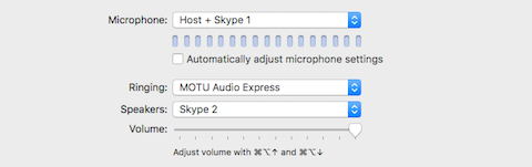
Once again we revert back to independent Virtual Devices created in Loopback for the configuration of this Skype instance. The Host + Skype 1 device is essentially output 5 in the configured DAW. It passes the Host + Skype Client 1 audio to this running instance of Skype.

[Speakers: Skype 2] is mapped to input 6, previously assigned in the DAW’s configured Session.

Recording in the Box

After launching and configuring the Skype instance(s), arm the DAW’s Host, Skype 1, and Skype 2 audio tracks for recording. Connect with the independent Skype participants. Both participants will be able to converse with each other + the Host. Recording the Session will supply discrete audio files for each participant on their respective tracks.

External Recording

In the I/O Matrix diagram you will notice the availability of two sets of stereo outputs (9+10 , 11+12). They represent the Line Outputs and the S/PDIF output on the Motu Interface. Remember the Interface is a Subdevice within the defined Aggregate Device. As a result the noted inputs and outputs are available within the DAW Session for patching.

Also notice the last two Channel Strips (Red) displayed in the Session mixer. They are Auxiliary Input Channel Strips. Their inputs are assigned to the Skype 1 and Skype 2 output Buses. Each Channel Strip output is mapped to corresponding Motu Interface Line Outputs and finally patched to the L+R inputs of an external solid state stereo recorder.

In this particular example only the Skype Participants will be recorded externally. My intension is to engineer Sessions containing two remote clients. In this case it’s a viable solution for out of the box Session recording.

Inserts

You will notice a few additional Audio Plugins inserted on various Channel Strips. A Mix Bus Compressor and a Limiter are inserted on the Mix Offset Channel Strip.

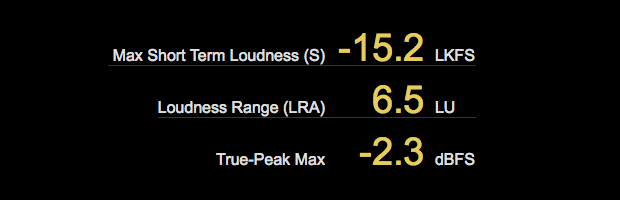
The Inserts located on the Master Fader are post fader. Here I’ve inserted the Clarity M routing plugin. This passes the signal to an external (hardware) Loudness Meter via USB.

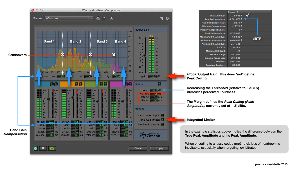
Finally I’ve inserted Limiters on each of the external recorder Buses. Again they are set to maintain maximum headroom, and only exist to prevent unexpected signal level overload before the audio reaches the recorder.

Of course Plugin implementation in general will be subjective.

Notes

The complexity of the Session can be customized or even minimized to suit your needs. Basic requirements include a properly configured Aggregate I/O, 3 audio tracks capable of recording, 2 Aux Sends, and a Master Fader. The dual Skype requirement is necessary and straightforward.

It is possible to add support for additional running Skype clients. This will require additional (mono) Loopback Pass-Thru Virtual Devices, and further customization of the Aggregate Audio Device + DAW Session.

I defined custom Incoming Connection Ports for each Skype Instance. This option is available in Skype Preferences/Advanced. Port Mapping was managed in my Router’s configuration utility.

I closely monitored System Resources throughout testing and checked for potential deficiencies. Pro Tools performed well with no issues. Each running instance of Skype displayed less than 14% CPU usage. Memory consumption was equally low. Note my Quad 2.8 GHz Mac Pro has 32 gigs of RAM and four dedicated media drives.

Undoubtedly someone will state this implementation is “much too complicated for the common Podcaster,” or even “Broadcaster.” With respect I’m not necessarily targeting novices. Regardless, you will most certainly require skills and experience in DAW and I/O signal routing.

Please note a Mix-Minus feed in general is not some sort of revelation. It’s pretty basic stuff. You’ll need a full understanding of it as well.

If you have questions I am happy to help. If you would like to participate in a test, ping me. If you are overwhelmed please revert to a service such as Zencastr.

-paul.

Understanding Pan Mode Options

Adobe Audition and Logic Pro X include Pan Mode preference options that determine track output gain for center panned mono clips included in stereo sessions. These options are often the source of confusion when working with a combination of mono and stereo clips, especially when clips are pre-Loudness Normalized prior to importing.

In Audition, the Left/Right Cut (Logarithmic) option retains center panned mono clip gain. The -3.0 dB Center option, which by the way is customizable – will attenuate center panned mono clip gain by the specified dB value.

For example if you were targeting -16.0 LUFS in a stereo session using a combination of pre-Loudness Normalized clips, and all channel faders were set to unity – the imported mono clips need to be -19.0 LUFS (Integrated). The stereo clips need to be -16.0 LUFS (Integrated). The Left/Right Cut Pan Mode option will not alter the gain of the center panned mono clips. This would result in a -16.0 LUFS stereo mixdown.

Conversely the -3.0 dB Center Pan Mode option will apply a -3 dB gain offset (it will subtract 3 dB of gain) to center panned mono clips resulting in a -19.0 LUFS stereo mixdown. In most cases this -3 LU discrepancy is not the desired target for a stereo mixdown. Note 1 LU == 1 dB.

As stated Logic Pro X provides a similar level of Pan Mode flexibility. I’ve also tested Reaper, and it’s options are equally flexible.

Pro Tools

Pro Tools Pan Mode support (they call it Pan Depth) is somewhat restricted. The preference is limited to Center Pan Mode, with selectable dB compensation options (-2.5 dB, -3.0 dB, -4.5 dB, and -6.0 dB).

There are several ways to reconstitute the loss of gain that occurs in Pro Tools when working with center panned mono clips in stereo sessions. One option would be to duplicate a mono clip and place each instance of it on hard-panned discrete mono tracks (L+R respectively). Routing the mono tracks to a stereo output will reconstitute the loss of gain.

A second and much more efficient method is to route all individual instances of mono session clips to a stereo Auxiliary Input, and use it to apply the necessary compensating gain offset before the signal reaches the stereo Master Output. The gain offset can be applied using the Aux Input channel fader or by using an inserted gain trim plugin. Stereo clips included in the session can bypass this Aux and should be directly routed to the stereo Master Output. In essence stereo clips do not require compensation.

Example Session

Have a look at the attached Pro Tools session snapshot. In order to clearly display the signal path relative to it’s gain, I purposely implemented Pre-Fader Metering.

pt-pan_small

Notice how the mono spoken word clip included on track 1 is routed (by way of stereo Bus 1-2) to a stereo Auxiliary Input track (named to Stereo). Also notice how the stereo signal level displayed by the meters on the Stereo Auxiliary Input track is lower than the mono source that is feeding it. The level variation is clear due to Pre-Fader Metering. It is the direct result of the session’s Pan Depth setting that is subtracting -3dB of gain on this center panned mono track.

Next, notice how the signal level on the Master Output has been reconstituted and is in fact equal to the original mono source. We’ve effectively added +3dB of gain to compensate for the attenuation of the original center panned mono clip. The +3dB gain compensation was applied to the signal on the Auxiliary Input track (via fader) before routing it’s output to the stereo Master Output.

So it’s: Center Panned mono resulting in a -3dB gain attenuation —>> to a stereo Aux Input with +3dB of gain compensation —>> to stereo Master Output at unity.

In case you are wondering – why not add +3dB of gain to the mono clip and bypass all the fluff? By doing so you would be altering the native inherent gain structure of the mono source clip, possibly resulting in clipping. My described workflow simply reconstitutes the attenuated gain after it occurs on center panned mono clips. It is all necessary due to Pro Tool’s Pan Depth methods and implementation.

-paul.

Quantifying Podcast Audio Dynamics

I’ve discussed the reasons why there is a need for revised (optimized) Loudness Standards for Internet and Mobile audio distribution. Problematic (noisy) consumption environments and possible device gain deficiencies justify an elevated Integrated Loudness target. Highly dynamic audio complicates matters further.

In essence audio for the Internet/Mobile platform must be perceptually louder on average compared to audio targeted for Broadcast. The audio must also exhibit carefully constrained dynamics in order to maintain optimized intelligibility.

The recommended Integrated Loudness targets for Internet and Mobile audio are -16.0 LUFS for stereo files and -19.0 LUFS for mono. They are perceptually equal.

In terms of Dynamics, I’ve expressed my opinion regarding compression. In my view spoken word audio intelligibility will be improved after careful Dynamic Range Compression is applied. Note that I do not advocate aggressive compression that may result in excessive loudness and possible quality degradation. The process is a subjective art. It takes practice with accessibility to well designed tools along with a full understanding of all settings.

Dynamic-480

I thought I would discuss various aspects of Podcast audio Dynamics. Mainly, the potential problematic significance of wide Dynamics and how to quantify aspects as such using various descriptors and measurement tools. I will also discuss the benefits of Dynamic Range management as a precursor to Loudness Normalization. Lastly I will disclose recommended benchmarks that are certainly not requirements. Feel free to draw your own conclusions and target what works best for you.

Highly Dynamic Audio in Noisy Environments

At it’s core extended or Wide Dynamic Range describes notable disparities between high and low level passages throughout a piece of audio. When this is prevalent in a spoken word segment, intelligibility will be compromised – especially in situations where the listening environment is less than ideal.

For example if you are traveling below Manhattan on a noisy subway, and a Podcast talent’s delivery is inconsistent, you may need to make realtime playback volume adjustments to compensate for any inconsistent high and low level passages.

As well – if the Integrated Loudness is below what is recommended, the listening device may be incapable of applying sufficient gain. Dynamic Range Compression will reestablish intelligibility.

From a post perspective – carefully constrained dynamics will provide additional headroom. This will optimize audio for further down stream processing and ultimately efficient Loudness Normalization.

Dynamic Range Compression and Loudness Normalization

I would say in most cases successful Loudness Normalization for Broadcast compliance requires nothing more than a simple subtractive gain offset. For example if your mastered piece checks in at -20.0 LUFS (stereo), and you are targeting R128 (-23.0 LUFS Integrated), subtracting -3 LU of gain will most likely result in compliant audio. By doing so the original dynamic attributes of the piece will be retained.

Things get a bit more complicated when your Integrated Loudness target is higher than the measured source. For example a mastered -20.0 LUFS piece will require additional gain to meet a -16.0 LUFS target. In this case you may need to apply a significant amount of limiting to prevent the Maximum True Peak from exceeding your target. In essence without safeguards, added gain may result in clipping. The key is to avoid excessive limiting if at all possible.

How do we optimize audio before a gain offset is applied?

I recommend applying a moderate to low amount of (global) final stage Dynamic Range Compression before Loudness Normalization. When processing highly dynamic audio this final stage compression will prevent instances of excessive limiting. The amount of compression is of course subjective. Often a mere 1-2 dB of gain reduction will be sufficient. Effectiveness will always depend on the attributes of the mastered source audio before L.Normalizing.

I carefully manage spoken word dynamics throughout client project workflows. I simply maintain sufficient headroom prior to Loudness Normalization. In most cases I am able to meet the intended Integrated Loudness and Maximum True Peak targets (without limiting) by simply adding gain.

RX Loudness Control

By design iZotope’s RX Loudness Control also applies compression in certain instances of Loudness Normalization. I suggest you read through the manual. It is packed with information regarding audio loudness processing and Loudness Normalization.

RX-LC_site

iZotope states the following:

“For many mixes, dynamics are not affected at all . This is because only a fixed gain is required to meet the spec . However, if your mix is too dynamic or has significant transients, compression and/or limiting are required to meet Short-term/Momentary or True Peak parts of the spec.”

“RX Loudness Control uses compression in a way that preserves the quality of your audio . When needed, a compressor dynamically adjusts your audio to ensure you get the 
best sound while remaining compliant . For loudness standards that require Short-term 
or Momentary compliance, the compressor is engaged automatically when loudness exceeds the specified target.”

It’s a highly recommended tool that simplifies offline processing in Pro Tools. Many of it’s features hook into Adobe’s Premiere Pro and Media Encoder.

LRA, PLR, and Measurement Tools

So how do we quantify spoken word audio dynamics? Most modern Loudness Meters are capable of calculating and displaying what is referred to as the Loudness Range (LRA). This particular descriptor is displayed in Loudness Units (LU’s). Loudness Range quantifies the differences in loudness measurements over time. This statistical perspective can help operators decide whether Dynamic Range Compression may be necessary for optimum intelligibility on a particular platform. (Note in order to prevent a skewed measurement due to various factors – the LRA algorithm incorporates relative and absolute threshold gating. For more information: refer to EBU Tech doc 3342).

I will say before I came across sort of rule of thumb (recommended) guidelines for Internet and Mobile audio distribution, the LRA in the majority of the work that I’ve produced over the years hovered around 3-5 LU. In the highly regarded article Audio for Mobile TV, iPad and iPod, the author and leading expert Thomas Lund of TC Electronic suggests an LRA not much higher than 8 LU for optimal Pod Listening. Basically higher LRA readings suggest inconsistent dynamics which in turn may not be suitable for Mobile platform distribution.

Some Loudness Meters also display the PLR descriptor, or Peak to Loudness Ratio. This correlates with headroom and dynamic range. It is the difference between the Program (average) Loudness and maximum amplitude. Assuming a piece of audio has been Loudness normalized to -16.0 LUFS along with an awareness of a True Peak Maximum somewhere around -1.0 dBTP, it is easy to recognize the general sweet spot for the Mobile platform ->> (e.g. a PLR reasonably less than 16 for stereo).

Note that heavily compressed or aggressively limited (loud) audio will exhibit very low PLR readings. For example if the measured Integrated Loudness of a particular program is -10.0 LUFS with a Maximum True Peak of -1.0 dBTP, the reduced PLR (9) clearly indicates aggressive processing resulting in elevated perceptual loudness. This should be avoided.

If you are targeting -16.0 LUFS (Integrated), and your True Peak Maximum is somewhere between -1.0 and -3.0 dBTP, your PLR is well within the recommended range.

In Conclusion

An optimal LRA is vital for Podcast/Spoken Word distribution. Use it to gauge delivery consistency, dynamics, and whether further optimization may be necessary. At this point in time I suggest adhering to an LRA < 7 LU for spoken word.

LRA Measurements may be performed in real time using a compliant Loudness Meter such as Nugen Audio’s VisLM 2, TC Electronic’s LM2n Loudness Radar, and iZotope’s Insight (also check out the Youlean Loudness Meter). Some meters are capable of performing offline measurements in supported DAWs. There are a number of stand alone third party measurement options available as well, such as iZotope’s RX7 Advanced Audio Editor, Auphonic Leveler, FFmpeg, and r128x.

-paul.

***Please note I personally paid for my RX Loudness Control license and I have no formal affiliation with iZotope.

Public Radio Loudness Compliance

PRSS (Public Radio Satellite System) recently published Loudness Standardization parameters intended for contributing producers:

[– Target Loudness: Integrated loudness shall be -24 LUFS per program segment with a variance of ±2 LU. This will apply to speech and/or music elements.

[– Maximum Peak Level: Shall be no higher than -3 dBFS for sample peaks and shall be no higher than -2 dBTP for True Peaks.

To supplement the published standards, my twitter acquaintance and fellow Loudness advocate Rob Byers posted The Audio Producer’s Guide to Loudness on Transom.org.

The article documents the basics of Loudness Meters, measurement descriptors, and mixing best practices. It’s a viable guide for anyone planning to submit compliant audio for Public Radio distribution. Incidentally Rob is the Interim Director of Broadcast and Media Operations with Marketplace at American Public Media.

Anyway … I’d like to share my personal perspective regarding the differences between real time compliance mixing vs. compliance processing. I’m confident my subjective insight will prove to be useful for Public Radio Producers targeting the PRSS spec.

Internet/Mobile vs. Broadcast

I’ve stated that targeted (Integrated/Program) Loudness for Radio/Broadcast differs from what I consider suitable for audio distributed on the Internet. This includes streaming audio, video, and Podcasts. Basically audio mixed and/or Loudness Normalized to -23.0/-24.0 LUFS, targeted to comply with a Broadcast spec. is simply not loud enough for Internet distribution. This is due to various aspects of consumption, including device deficiencies and problematic ambiance in less than ideal listening environments. The Integrated Loudness target for Internet/Mobile audio is -16.0 LUFS with allowance for a reasonable deviation. True Peaks should not exceed -1.0 dBTP in lossy files. Some institutions suggest additional headroom.

Mixing for Compliance

I rarely mix audio in real time while attempting to meet Integrated and True Peak compliance targets. This method is acceptable. However there are a few caveats.

First, in order to arrive upon an accurate representation of Integrated Loudness, audio mixes must be measured in their entirety. You cannot spot check a few passages of a mix and estimate this descriptor. Needless to say this can be a time consuming process.

Secondly, in my view real time mixing for compliance is tedious and potentially inaccurate. What I recommend is to use both the Short Term and Integrated Loudness descriptors to sort of gauge the current state of the mix as playback progresses and ends. Once the mix has concluded – simply apply a global Gain Offset to the entire mix. This will shift the Integrated Loudness to your intended target. This is essentially one way to apply Loudness Normalization.

For example if a concluded mix checks in at -20.0 LUFS, and you are targeting -24.0 LUFS, prior to bouncing, a -4LU (dB) global Gain Offset would bring the mix into spec. (The process is discussed in this video highlighting the TC Electronic Loudness Radar Meter included in Adobe Audition and Premiere Pro. Of course any compliant Loudness Meter would be suitable).

By the way let’s not forget the importance of True Peak compliance for any standard. This descriptor will also need to be monitored and dealt with accordingly while mixing.

Trust Your Ears!

This second (and preferred) method of Loudness Normalization requires proper use of the most important tool(s) available to all of us in any mixing or post production environment … our ears. Producers need to learn how to take advantage of natural perception and also apply thoughtful processing to session clips with the intent to achieve a well balanced, good sounding mix. In doing so the use of a Loudness Meter becomes much less of a distraction.

Of course the presence of an inserted meter is a necessity, and it’s descriptors will (over time) display a clear indication of the state of the mix. Trust your ears!

Off-line Loudness Normalization

The workflow that I’m about to describe will reward producers with Loudness compliance flexibility throughout a mixing session. The key is upon completion, the mixed (and exported) audio will be processed off-line resulting in 100% compliance.

As noted, the global Gain Offset method for Loudness Normalization requires knowledge of existing Integrated Loudness prior to applying the necessary adjustments. The following variation shares the same requirement. However the Integrated Loudness and True Peak of the mixed-down audio will be calculated off-line as opposed real time. Let me stress the existing Integrated Loudness must be realized before we can move forward with any form of compliance processing. We will be targeting the PRSS specifications noted above.

FFMpeg:Cross Platform Support

There are many ways to measure audio off-line. The most accessible and economical cross-platform tool is the FFmpeg binary. Indeed this is a Command Line utility. Don’t fret! It’s not that big of a deal. You can easily download a pre-complied binary compatible with your current operating system. You simply point your command line syntax to the location of the binary, key in the path to the location of the file to be measured, and fire away.

Below is example syntax for Loudness Measurement. In this particular instance I point to the binary stored in a root, system wide folder. If you are running a Mac, it may be easier to simply place the binary on your Desktop. In this case you would point to the binary like this: ~/Desktop/ffmpeg … then continue with the remaining displayed syntax, replacing yourSourceFile.wav with the actual path of the file to be measured.

ffmpeg_syntax

And here are the results. Notice the -19.9 LUFS Integrated Loudness (I), and the 1.8 dBFS (dBTP) True Peak (open the image for an extended view).

ffmpeg-small

The PRSS spec. calls for -24.0 LUFS Integrated Loudness with Sample Peaks not exceeding -3.0 dB and True Peaks not exceeding -2.0 dBTP. In this measured example the audio is roughly +4LU louder than it should be and it is obviously clipped with it’s True Peak well above 0dBFS.

Setting Up The Normalization Session

In your preferred DAW, create a new stereo session and do the following:

[– Add a Stereo Audio Track, two Stereo AUX Input Channels (primary/secondary), and a Master Fader.

[– Route the Audio Track’s output to the input of the primary Aux Input Channel.

[– On the primary Aux Input Channel – first insert a Gain Trim plugin. Then insert a True Peak Limiter.

[– Now route the output of the primary Aux Input Channel to the input of the secondary Aux Input Channel.

[– Insert a second instance of a Gain Trim plugin on the secondary Aux Input Channel.

[– Route the processed signal to the Master Fader.

[– Set the True Peak Ceiling on the Limiter to -3.5dBTP. Set the Gain Trim inserted on the secondary Aux Input Channel to +1dB. Note that these settings are static and will never change.

Save the session as a Template.

Here is an example of how I do this in Pro Tools. Note that I have additional plugins inserted on the sessions’s Aux Input Channels. They are in fact deactivated. Please disregard them. I was using this example session for testing, using duplicate sets of plugins for various parameter adjustments. (click to enlarge).

pt-(-24)_620

Making it Work

Using the measured audio displayed above, note the Integrated Loudness (-19.9 LUFS). All you need to do is calculate an initial Gain Offset. This is the difference between the measured Integrated Loudness and -25.0. Add the mixed-down audio into the session’s Audio Track, and set the Gain Trim plugin inserted on the Primary Aux Input Channel to the calculated Gain Offset.

Bounce and you’re done.

Note that the initial Gain Offset will always be determined by calculating the difference between existing Integrated Loudness and -25.0. Once the core session Template is saved, subsequent use is simple: Measure mixed-down audio – Import audio into session – Calculate Gan Offset – Apply Offset to Primary Gain Trim – Bounce.

This is the fourth paragraph …

TP-620

Additional text …

Adobe Audition Multiband Compressor

I thought I’d clear up a few misconceptions regarding the Multiband Compressor bundled in Adobe Audition. Also, I’d like to discuss the infamous “Broadcast” preset that I feel is being recommended without proper guidance. This is an aggressive preset that applies excessive compression and heavy limiting resulting in processed audio that is often fatiguing to the listener.

audition-multi-480

The Basics

The tool itself is “Powered by iZotope.” They are a well respected audio plugin and application development firm. Personally I think it’s great that Adobe decided to bundle this processor in Audition. However, it is far from a novice targeted tool. In fact it’s pretty robust.

What’s interesting is it’s referred to as a “Multiband Compressor.” This is slightly misleading, considering the processor includes a Peak Limiter stage along with it’s advertised Multiband Compressor. I think Dynamics Processor would be a more suitable name.

Basically the multi-band Compressor includes 3 adjustable crossovers, resulting in 4 independent Frequency Bands. Each Band includes a discrete Compressor with Threshold, Gain Compensation, Ratio, Attack, and Release settings. Bands can be soloed or bypassed.

There is global Peak Limiter module located to the right of the Compressor settings. This module may be activated or bypassed. Without a clear understanding of the supplied settings for the Limiter, you run the risk of generating excessive loudness when processing audio. I’m referring to a substantial increase in perceived loudness.

The Limiter Parameters

The Threshold is the limiting trigger. When the input signal surpasses it, limiting is activated. The Margin is what defines the Peak Ceiling. As you decrease the Threshold, the signal is driven up to and against the Margin resulting in an increase in average loudness. This also results in dynamic range reduction.

Activating the “Brickwall Limiter” feature in the supplemental Options module will ensure accurate Margin compliance. In essence you will be implementing Hard Limiting. Deactivating this option may result in “overs” and/or peaks that exceed the specified Margin.

The bundled Broadcast preset defaults the Limiter Threshold setting to -10.0 dB with a Margin of -0.1 dBFS. Any alternative Threshold settings are of course subjective. I’m suggesting that it may be a good idea to ease up on this default Threshold setting. This will result in less aggressive limiting and a reduction of average levels.

I’m also suggesting that the default Margin setting of -0.1 is not recommended in this context. I would set this to -1.0 dBFS or lower (-1.5 dBFS, or even -2.0 dBFS).

Please note this is not a True Peak Limiter. Your processed lossless audio file has the potential to loose headroom when and if it is converted to a lossy codec such as MP3.

At this point I suggest no changes should be made to the Attack and Release settings.

The Compressors

We cannot discount additional settings included in the Broadcast preset that are contributing to the aggressive processing. If you examine the Ratio settings for each independent compression module, 3:1 is the highest set Ratio. The predefined Ratios are fairly moderate and for starters require no adjustment.

However, notice the Threshold settings for each compression module as well as the Gain Compensation setting in Module (band) 4 (+3 dB).

First, the low Threshold settings result in fairly aggressive compression per band. Also, the band 4 gain compensation is generating a further increase in average level for that particular band.

Again the settings and any potential adjustments are subjective. My recommendation would be to experiment with the Threshold settings. Specifically, cut back by reducing all Thresholds while maintaining their relative relationship. Do this by activating the “Link Band Controls” setting located in the supplemental Limiter Options.

View the red Gain Reduction meters included in each module. Monitor the amount of attenuation that occurs with the default Threshold settings. Compare initial readings with the gain reduction that occurs after you make your adjustments. Your goal is to ease up on the gain reduction. This will result in less aggressive compression. Remember to use your ears!

Output

An area of misinformation for this processor is the purpose of the Output Gain adjustment, located at the far upper right of the interface. Please note this setting does not define the Peak Ceiling! Remember – it is the Margin setting in the Limiter module that defines your Ceiling. The Output Gain simply adds or cuts global output level after compression. Think of if it as Global Gain compensation.

To prove my point, I dug out a short video demo that I created sometime last year for a community member.

With the Broadcast preset selected, and the Output Gain set to -1.5 dBFS – the actual output Peak Amplitude surpasses -1.5 dBFS, even with the Brickwall option turned ON. This reading is displayed numerically above the Output Gain meter(s) in real time.

In the second pass of the test I set the Output Gain to 0 dBFS. I then set the Limiter Margin to -1.5 dBFS. As the audio plays through you will notice the output is limited to and never surpasses -1.5 dBTP. Just keep your eye on the numerical, realtime display.

Video Demo Link

I purposely omitted any specific references to Attack and Release settings. They are the source for a future discussion.

DeEsser?

Here’s an alternative use recommendation for this Adobe Multiband Compressor: DeEssing.

Use the Spectrum Analyzer to determine the frequency range where excessive sibilant energy occurs. Set two crossovers to encapsulate this range. Bypass the remaining associated compression modules. Tweak the remaining active band compression settings thus allowing the compressor to attenuate the problematic sibilant energy.

If you find the supplied Spectrum Analyzer difficult to read, consider using a third party option with higher resolution to perform your analysis.

Conclusion

Please note – in order to get the most out of this tool, you really need to learn and understand the basics of dynamics compression and how each setting will affect the source audio. More importantly, when someone simply suggests the use of a preset, take it with a grain of salt. More than likely this person lacks a full understanding of the tool, and may not be capable of providing clear instructional guidance for all functions. It’s a bad mix – especially when charging novices big bucks for training.

By the way, nothing wrong with being a novice. The point is paid consultants have an obligation to provide expert assistance. Boiler plate suggestions serve no purpose.

-paul.

dbx 286s: Beyond The Basics …

The dbx brand has been a favorite of mine since the late 1970’s. My first piece of dbx kit was a stand-alone noise reduction unit that I coupled with an old Teac Reel to Reel Tape Deck. Through the years I’ve owned various EQ’s and Dynamics processors, including the highly regarded 160A Compressor. I purchased mine in 2006.

160a-small

In January 2011 I was skimming through eBay listings looking for a dbx 286A Microphone Preamp Processor. At the time I had heard the original 286 model was co-designed by Bob Orban, and both models were widely used in Radio Broadcast facilities. I found it interesting that Radio Engineers would use a piece of gear that was not only cheap in terms of cost – but unconventional in terms of controls.

286A-small

One piece was available on eBay, supposedly used for 4 hours at a party in Hollywood Hills California, and then boxed for resale. The seller had a positive reputation, so I grabbed it for $115. Upon arrival it’s condition was as described, and it’s been in my rack ever since.

The 286/286A has evolved into the 286s, quite frankly an outright steal priced at $199. Due to it’s straight forward approach and affordable price, the Podcasting community has embraced it and often classifies it as “drool-worthy.” Pretty amusing.

286-small

In this article I am going to focus on the attributes of the Compressor stage and the De-Esser. I will demystify the DeEsser and discuss the importance of the Output (Gain) Compensation setting.

Unconventional

I mentioned the processor is unconventional. For example the Compressor’s Drive and Density settings essentially replace the Threshold, Ratio, Attack, and Release controls present on most Compressors.

The De-Esser requires a user defined High-Pass Frequency designation and Threshold setting to reduce excessive sibilance. Setup can be time consuming due to the lack of any visual representation of problematic energy in need of attenuation.

Compressor:Drive

Compression results depend on the level (and dynamics) of the incoming signal and corresponding settings. On a conventional compressor the Threshold monitors the incoming signal. When the signal surpasses the Threshold, processing engages and gain reduction is activated. The Ratio determines the amount of gain reduction. The Attack will affect how aggressively (or the speed at which) gain reduction initializes and ultimatly reaches maximum attenuation. The Release will control the speed of the transition from full attenuation – back to the original level

The Drive control on the 286s determines the amount of gain reduction (compression) applied to the incoming signal. Higher settings will increase the input signal level resulting in more aggressive compression (and noise).

How much gain reduction should you shoot for? Well that’s subjective. I would recommend experimenting with 6-12dB of gain reduction. Of course results will vary due to obvious variables (mic selection, preamp level, etc.)

Compressor:Density

When using a compressor to process spoken word, improper Release settings can result in choppiness, often referred to as pumping. The key is to have the gain reduction occurrences smoothly transition between instances of audible sound and natural pauses (silence).

The 286s uses a variable program dependent Release. In the event you feel (and hear) the necessity to speed up or slow down the program dependent Release – the Density control will come in handy.

Note the Density scale on the 286s is again somewhat unconventional. On a typical dynamics processor – setting the Release full counter-clockwise would result in a very fast Release. As the setting is adjusted clockwise, the Release duration is extended. The scale usually transitions from milliseconds to full seconds.

On the 286s, think of Density as a linear speed controller, where “1” (counter-clockwise) is slow and “10” (full clockwise) is fast.

For normal speech I recommend experimenting with the Density set between 3 and 5.

The De-Esser

If you check around you will notice a wide range of references regarding the frequency range where sibilance generally occurs. In reality there are many variables. Each instance of sibilance will need to be accurately identified and addressed accordingly.

The 286s De-Esser uses a variable high-pass filter. This instructs the processor where to initiate the attenuation of problematic energy. This Frequency control has a range of 800Hz-10kHz. The user manual states ” … settings between 4-8kHz will yield the best results for vocal processing.” This is good starting point. However proper setup requires time consuming arbitrary tweaking that may result in a low level of accuracy. A visual representation of the frequency range of the excessive sibilant energy will solve this problem. Once you identify the frequencies and/or range where most of the energy is present, setting the Frequency on the 286s will be demystified.

The De-Esser’s Threshold setting controls the amount of attenuation (sensitivity) and will remain constant as the input level changes.

Have a look at the spectral analysis below:

sibilance-small

Notice the excessive energy in the 2-6kHz range (Frequency Range is represented on the X axis). For this particular segment of audio I would initially set the Frequency control on the 286s to 5kHz. Next I would adjust the Threshold until the sibilant energy is attenuated. I would then sweep the Frequency setting within the visual range of the sibilant energy and fine tune both settings until I achieve the most pleasing results. The key is not to over do it. Heavy attenuation will suppress vital energy and remove any hint of natural presence and sparkle.

To perform this analysis excersize – set the Threshold setting on the 286s to OFF. Pass the output of the processor to your DAW of choice and perform a real time spectral analysis of your voice using a software plugin the includes a Spectrum Analyzer. You can use any supported EQ plugin with it’s controls bypassed. You can also use something like the free (AU/VST) Span plugin by Voxengo (note that Span is CPU intensive).

Output Gain Compensation

Gain Compensation is an integral element of Audio Compression. It’s intent is to offset the gain reduction that occurs when audio is compressed. It is often referred to as Make-up Gain. When this gain offset is applied to compressed audio, the perceived, average level of the audio is increased. Excessive Make-up Gain can sometimes elevate noise that may have been previously inaudible at lower average levels.

Earlier I discussed how an elevated Drive control setting on the 286s will increase the input signal of low level source audio. In doing so you may initiate a suitable amount of compression. However you also run the risk of a noticeable increase in noise. In this particular scenario, try setting the Output Gain on the 286s to a negative value to offset the gain (and noise) that may have been introduced by the Drive setting.

Conclusion

I think it’s important to first learn the basics of Audio Compression from a conventional perspective. In doing so you will find it easier to get the most out of the unconventional controls on the dbx 286s, especially Drive and Density.

And let’s not forget that De-Essing is really nothing more than frequency band compression that will attenuate problematic energy. Establishing a visual reference to the energy will simplify the process of accurate correction.

-paul.

Asymmetric Waveforms: Should You Be Concerned?

In order to understand the attributes of asymmetric waveforms, it’s important to clarify the differences between DC Offset and Asymmetry …

Waveform Basics

A waveform consists of both a Positive and Negative side, separated by a center (X) axis or “Baseline.” This Baseline represents Zero (∞) amplitude as displayed on the (Y) axis. The center portion of the waveform that is anchored to the Baseline may be referred to as the mean amplitude.

wf-480

DC Offset

DC Offset occurs when the mean amplitude of a waveform is off the center axis due to differing amounts of the signal shifting to the positive or negative side of the waveform.

One common cause of this shift is when faulty electronics insert a DC current into the signal. This abnormality can be corrected in most file based editing applications and DAW’s. Left uncorrected, audio with DC Offset will exhibit compromised dynamic range and a loss of headroom.

Notice the displacement of the mean amplitude:

dc-offset-ex-480-png

The same clip after applying DC Offset correction. Also, notice the preexisting placement of (+/-) energy:

dc-offset-removed-480

Asymmetry

Unlike waveforms that indicate DC Offset, Asymmetric waveform’s mean amplitude will reside on the center axis. However the representations of positive and negative amplitude (energy) will be disproportionate. This can inhibit the amount of gain that can be safely applied to the audio.

In fact, the elevated side of a waveform will tap the target ceiling before it’s counterpart resulting in possible distortion and the loss of headroom.

High-pass filters, and aggressive low-end processing are common causes of asymmetric waveforms. Adding gain to asymmetric waveforms will further intensify the disproportionate placement of energy.

In this example I applied a high-pass filter resulting in asymmetry:

asymm-matural-480

Broadcast Chains

Broadcast engineers closely monitor positive to negative energy distribution as their audio passes through various stages of processing and transmission. Proper symmetry aides in the ability to process a signal more effectively downstream. In essence uniform gain improves clarity and maximizes loudness.

Podcasts

In spoken word – symmetry allows the voice to ride higher in the mix with a lower risk of distortion. Since many Podcast Producers will be adding gain to their mastered audio when loudness normalizing to targets, the benefits of symmetric waveforms are obvious.

If an audio clip’s waveform(s) are asymmetric and the audio exhibits audible distortion and/or a loss of headroom, a Phase Rotator can be used to reestablish proper symmetry.

Below is a segment lifted from a distributed Podcast (full zoom out). Notice the lack of symmetry, with the positive side of the waveform limited much more aggressively than the negative:

podcast-asymm-480

The same clip after Phase Rotation:

asymm-podcas-fixed-480

(I processed the clip above using the Adaptive Phase Rotation option located in iZotope’s RX 4 Advanced Channel Ops module.)

In Conclusion

Please note that asymmetric waveforms are not necessarily bad. In fact the human voice (most notably male) is often asymmetric by nature. If your audio is well recorded, properly processed, and pleasing to the ear … there’s really no need to attempt to correct any indication of asymmetry.

However if you are noticing abnormal displacement of energy, it may be worth looking into. My suggestion would be to evaluate your workflow and determine possible causes. Listen carefully for any indication of distortion. Often a slight EQ tweak or a console setting modification is all that may be necessary to make noticeable (audible) improvements to your audio.

-paul.

Loudness Meter Descriptors …

In the recent article published on Current.org “Working Group Nears Standard for Audio Levels in PRSS Content”, the author states:

“Working group members believe that one solution may lie in promoting the use of Loudness Meters, which offer more precision by measuring audio levels numerically. Most shows are now mixed using peak meters, which are less exact.”

Peak Meters are exact – when they are used to display what they are designed to measure:Sample Peak Amplitude. They do not display an accurate representation of average, perceived loudness over time. They should only be used to monitor and ultimately prevent overload (clipping).

It’s great that the people in Public Radio are finally addressing distribution Loudness consistency and compliance. My hope is their initiative will carry over into their podcast distribution models. In my view before any success is achieved, a full understanding of all spec. descriptors and targets would be essential. I’m referring to Program (Integrated) Loudness, Short Term Loudness, Momentary Loudness, Loudness Range, and True Peak.

Loudness Meter

A Loudness Meter will display all delivery specification descriptors numerically and graphically. Meter descriptors will update in real time as audio passes through the meter.

Short Term Loudness values are often displayed from a graphical perspective as designed by the developer. For example TC Electronic’s set of meters (with the exception of the LM1n) display Short Term Loudness on a circular graph referred to as Radar. Nugen Audio’s VisLM meter displays Short Term Loudness on a grid based histogram. Both versions can be customized to suit your needs and work equally well.

meters-480

Loudness Meters also include True Peak Meters that display any occurrences of Intersample Peaks.

Descriptors

All Loudness standardization guidelines specify a Program Loudness or “Integrated Loudness” target. This time scaled descriptor indicates the average, perceived loudness of an entire segment or program from start to finish. It is displayed on an Absolute scale in LUFS (Loudness Units relative to Full Scale), or LKFS (Loudness Units K Weighted relative to Full Scale). Both are basically the same. LUFS is utilized in the EBU R128 spec. and LKFS is utilized in the ATSC A/85 spec. What is important is that a Loudness Meter can display Program Loudness in either LUFS or LKFS.

The Short Term Loudness (S) descriptor is measured within a time window of 3 seconds, and the Momentary Loudness (M) descriptor is measured within a time window of 400 ms.

The Loudness Range (LRA) descriptor can be associated with dynamic range and/or loudness distribution. It is the difference between average soft and average loud parts of an audio segment or program. This useful indicator can help operators decide whether dynamic range compression is necessary.

Gating

The specification Gate (G10) function temporarily pauses loudness measurements when the signal drops below a relative threshold, thus allowing only prominent foreground sound to be measured. The relative threshold is -10 LU below ungated LUFS. Momentary and Short Term measurements are not gated. There is also a -70 LUFS Absolute Gate that will force metering to ignore extreme low level noise.

Absolute vs. Relative

I mentioned that LUFS and LKFS are displayed on an Absolute scale. For example the EBU R128 Program Loudness target is -23.0 LUFS. For Podcast/Internet/Mobile the Program Loudness target is -16.0 LUFS.

There is also a Relative scale that displays LU’s, or Loudness Units. A Relative LU scale corresponds to an Absolute LUFS/LKFS scale, where 0 LU would equal the specified Absolute target. In practice, -23 LUFS in EBU R128 is equal to 0 LU. For Podcast/Mobile -16.0 LUFS would also be equal to 0 LU. Note that the operator would need to set the proper Program Loudness target in the Meter’s Preferences in order to conform.

ab-rel

LU and dB Relationship

1 LU is equal to 1 dB. So for example you may have measured two programs: Program A checks in at -20 LUFS. Program B checks in at -15 LUFS. In this case program B is +5 LU louder than Program A.

Placement

Loudness Meter plugins mainly support online (Real Time) measurement of an audio signal. For an accurate measurement of Program Loudness of a clip or mixed segment the meter must be inserted in the DAW at the very end of a processing chain, preferably on the Master channel. If the inserts on the Master channel are post fader, any change in level using the Master Fader will result in a global gain offset to the entire mix. The meter would then (over time) display the altered Program Loudness.

If your DAW’s Master channel has pre fader inserts, the Loudness Meter should still be inserted on the Master Channel. However the operator would first need to route the mix through a Bus and use the Bus channel fader to apply global gain offset. The mix would then be routed to the Master channel where the Loudness Meter is inserted.

If your DAW totally lacks inserts on the Master channel, Buses would need to be used accordingly. Setup and routing would depend on whether the buses are pre or post fader.

Some Loudness Meter plugins are capable of performing offline measurements in certain DAW’s on selected regions and/or clips. In Pro Tools this would be an Audio Suite process. You can also accomplish this in Logic Pro X by initiating and completing an offline bounce through a Loudness Meter.

-paul.

Podcasting System featuring the Allen & Heath XB-10 Console …

I continue to look around for a Broadcast Console that would be suitable to replace my trusty Mackie Onyx 1220i FW mixer. I was always aware of the XB-10 by Allen & Heath, although I did not pay much attention to it due to it’s use of pot-styled channel faders as opposed to sliding (long-throw) faders.

ah-mixer-480

Last evening I skimmed through the manual for the XB-10. Looking past the pot-styled fader issue this $799 console is packed with features that make it highly attractive. And it’s smaller than my Mackie, checking in at 13.2 inches wide x 10 inches deep. Allen & Heath also offers the XB-14-2 Console. It checks in at 15.2 inches wide x 18.3 inches deep with ample surface space for long-throw sliding faders. Bottom line is it’s larger than my Mackie and the size just doesn’t work for me.

XB-10: The Basics

Besides all the useful routing options, the XB-10 has a dedicated Mix-Minus channel that can be switched to receive the output of a Telephone Hybrid or the output of the bi-directional USB bus. In this case it would be easy to receive a Skype guest from a computer.

The console has latching On/Off switches on all input channels, supports pre-fader listening, and has built-in Compressors on channels 1-3. The manual states ” … the Compressor is optimized to reduce the dynamic range of the presenter microphone(s). Low signal levels are given a 10dB gain boost. Soft Knee compression activates at -20dBu, and higher level signals are limited.” Personally I would use a dedicated voice processor for the main presenter. However having the dynamics processing on-board is a useful feature, especially when adding additional presenters to the program mix.

The XB-10 is also equipped with an Output Limiter that can be used to ensure that the final mix does not exceed a predefined level. There is an activation switch located on the back panel of the device with a trim pot control to set the limiting threshold. If the Limiter is active and functioning, a front panel LED illuminates.

One other feature that is worth mentioning is the Remote Connector interface located on the back of the device. This can be used to implement CD player remote triggering, ON AIR light illumination, and external metering options.

I decided to design a system using the XB-10 as the controller that is suitable for flexible Podcast Production and Recording. Bear in mind I don’t have any of these system components on hand except for older versions of the dbx Voice Processor and the Telos Phone Hybrid. I also have a rack-mounted Solid State Recorder by Marantz, similar to the Tascam. I’m confident that all displayed components would work well together yielding excellent results.

Also note there are many ways to integrate these components within the system in terms of connections and routing. This particular design is similar in concept to how I have my current system set up using the components that I currently own (Click to Enlarge).

AH-system-480

System Design Concepts and Selections

The mic of choice is the Shure SM7B. The was the first broadcast style mic that I bought back in 2004 and it’s one of my prized possessions. As far as I’m concerned it’s the most forgiving broadcast mic available, with one caveat – it requires a huge amount of clean gain to drive it. Common +60dB gain trims on audio mixers will not be suitable, especially when setting the gain near or at it’s highest level. This will with no doubt result in problematic noise.

In my current system I plug my dynamic mic(s) into my dbx 286a Voice Processor (mic input) and then route the processor’s line output to a line input on one of the Mic channels on my Mackie mixer. By doing so I pick up an additional +40dB of available gain to drive the mic. Of course this takes a bit of tweaking to get the right balance between the gain setting on the processor and the gain setting on the Mackie. The key is not to max out either of the gain stages.

I’ve recreated this chain in the new design using the updated dbx 286s. In doing so the primary presenter gets the voice processor on her channel. If there is the necessity to expand the system by introducing a second presenter, I’ve implemented the Cloudlifter CL-1 gain stage between the mic and the console’s mic input on channel 2. The CL-1 will provide up to +20dB of additional clean gain when using any passive microphone. Finally I point to the availability of the on-board dynamics processor and consider this perfectly suitable for a second presenter.

I mentioned the XB-10 has a dedicated telephone interface channel with a built in mix-minus. Once again I’ve selected the Hx1 Digital Telephone Hybrid by Telos Systems for use in this system. The telephone interface channel can be set to receive an incoming telephone caller or something like the Skype output coming in from a computer. I’ve taken this a step further by also implementing an analog Skype mix-minus using the Console’s Aux Send to feed the computer input. The computer output is routed back into the Console on an available channel(s).

As noted the USB interface on the Console is bi-directional. One use case scenario would be to use the computer USB output to send sound effects and audio assets into the program mix. (I am displaying QCart for Mac as a possible option).

The rest is pretty self explanatory. I’m using the Monitor output bus to feed the studio speakers. The Console’s Main outputs are routed to the Tascam recorder, and it’s outputs are routed to an available set of inputs on the Console.

Like I said I’m fairly confident this system design would be quite functional and well suited for flexible Podcast Production and Recording.

In closing beginning in 2004 besides designing sort of generic systems based on various levels of cost and complexity, it was common for an aspiring Podcast Producer to reach out to me and ask for technical assistance with the components they purchased. In this case I would build detailed diagrams for the producer much the same as the example included in this post. A visual representation of system routing and configuration is a great way to expidite setup when and if the producer who purchased the gear is overwhelmed.

Note:

At one time I was providing a service where two individual participants were simultaneously calling into my studio for interview session recording. Since I had two dedicated phone lines and corresponding telephone hybrids, the participants were able two converse with each other using 2 Aux buses, in essence by creating two individual mix-minuses.

Here is the original diagram that I built in October 2006 that displays the routing of the callers via Aux sends:

dual-mm-480

Even though the XB-10 console contains a single Aux bus, a similar configuration may still be possible where an incoming caller from the telephone hybrid would be able to converse with a Skype guest, minus themselves. I need to read into this further before I am able to make a determination on whether this is supported.

Components:

[– Shure SM7B Broadcast Dynamic Microphone
[– Cloudlifter CL-1 Gain Stage
[– Allen & Heath XB-10 Broadcast Console
[– dbx 286s Voice Processor
[– Telos Hx1 Digital Telephone Hybrid
[– Tascam SS-R200 Solid State Recorder

Optional:

[– QCart for Mac OSX
[– KRK Rokit 5 Powered Studio Monitors

-paul.

Broadcast upTimer …

This is the updated version of a neat utility that I built about 5 years ago. Radio Stations sometime use what are referred to as upTimers to track live programs and air time. Hardware versions are available from main stream broadcast gear suppliers and can be quite expensive. In fact many of these devices can be remotely controlled using a console link. I thought a software version would be cool, so there you have it.

New options include the capability to set the timer Ceiling (60 or 90 minutes), HUD window interface, and date display. I decided to use a HUD window instead of a basic textured window. Clicking away from the running timer window does not affect clear visibility. The physical size of the window is now 840 x 365 pixels. This makes it easy to see from a distance.

I need to add the Sparkle Framework for automatic updating support before I release it …

-paul.

Update:

I replaced the current date with a Running Time display. Sparkle has been added as well …

You can download upTimer 2.0 here.